Vocabulary size and difference are semantic and linguistic concepts for mathematical and qualitative linguistics.
For example, Heaps’ law claims that the length of the article and vocabulary size are correlative. Still, after a certain threshold, the same words continue to appear without improving vocabulary size.
The Word2Vec uses Continuous Bag of Words (CBOW) and Skip-gram to understand the locally contextually relevant words and their distance to each other. At the same time, GloVe tries to use matrix factorization with context windows.
Zipf’s law is a complementary theory to Heaps’ law. It states that the most frequent and second most frequent words have a regular percentage difference between them.
There are other distributional semantics and linguistic theories in statistical natural language processing.
But “vocabulary comparison” is a fundamental methodology for search engines to understand “topicality differences,” “the main topic of the document,” or overall “expertise of the document.”
Paul Haahr of Google stated that it compares the “query vocabulary” to the “document vocabulary.”
David C. Taylor and his designs for context domains involve certain word vectors in vector search to see which document and which document subsection are more about what, so a search engine can rank and rerank documents based on search query modifications.
Comparing vocabulary differences between ranking web pages on the search engine results page (SERP) helps SEO pros see what contexts, concurrent words, and word proximity they are skipping compared to their competitors.
It is helpful to see context differences in the documents.
In this guide, the Python programming language is used to search on Google and take SERP items (snippets) to crawl their content, tokenize and compare their vocabulary to each other.
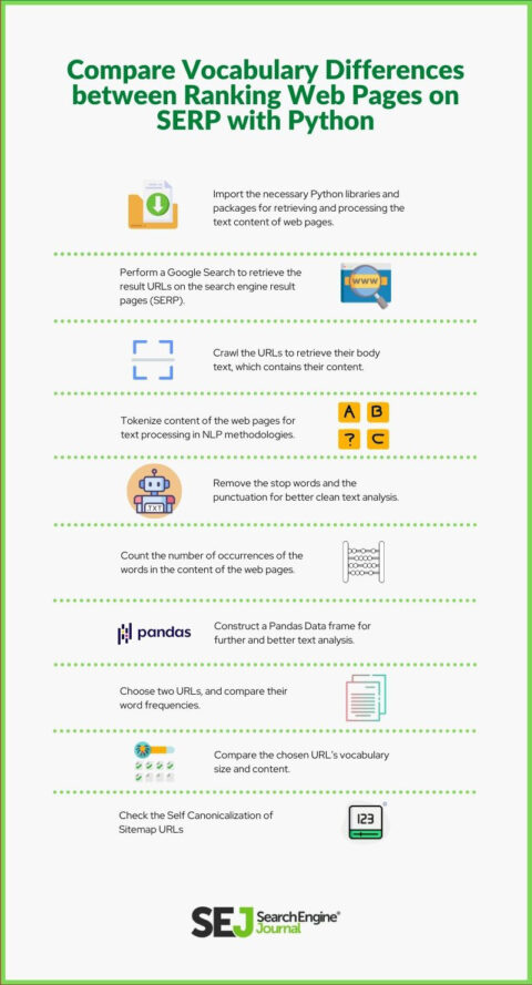
How To Compare Ranking Web Documents’ Vocabulary With Python?
To compare the vocabularies of ranking web documents (with Python), the used libraries and packages of Python programming language are listed below.
- Googlesearch is a Python package for performing a Google search with a query, region, language, number of results, request frequency, or safe search filters.
- URLlib is a Python library for parsing the URLs to the netloc, scheme, or path.
- Requests (optional) are to take the titles, descriptions, and links on the SERP items (snippets).
- Fake_useragent is a Python package to use fake and random user agents to prevent 429 status codes.
- Advertools is used to crawl the URLs on the Google query search results to take their body text for text cleaning and processing.
- Pandas regulate and aggregate the data for further analysis of the distributional semantics of documents on the SERP.
- Natural LanguageTool kit is used to tokenize the content of the documents and use English stop words for stop word removal.
- Collections to use the “Counter” method for counting the occurrence of the words.
- The string is a Python module that calls all punctuation in a list for punctuation character cleaning.
What Are The Steps For Comparison Of Vocabulary Sizes, And Content Between Web Pages?
The steps for comparing the vocabulary size and content between ranking web pages are listed below.
- Import the necessary Python libraries and packages for retrieving and processing the text content of web pages.
- Perform a Google search to retrieve the result URLs on the SERP.
- Crawl the URLs to retrieve their body text, which contains their content.
- Tokenize content of the web pages for text processing in NLP methodologies.
- Remove the stop words and the punctuation for better clean text analysis.
- Count the number of words occurrences in the web page’s content.
- Construct a Pandas Data frame for further and better text analysis.
- Choose two URLs, and compare their word frequencies.
- Compare the chosen URL’s vocabulary size and content.
1. Import The Necessary Python Libraries And Packages For Retrieving And Processing The Text Content Of Web Pages
Import the necessary Python libraries and packages by using the “from” and “import” commands and methods.
from googlesearch import search

from urllib.parse import urlparse

import requests

from fake_useragent import UserAgent

import advertools as adv

import pandas as pd

from nltk.tokenize import word_tokenize

import nltk

from collections import Counter

from nltk.corpus import stopwords

import string

nltk.download()
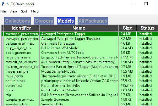
Use the “nltk.download” only if you’re using NLTK for the first time. Download all the corpora, models, and packages. It will open a window as below.
 Screenshot from author, August 2022
Refresh the window from time to time; if everything is green, close the window so that the code running on your code editor stops and completes.
If you do not have some modules above, use the “pip install” method for downloading them to your local machine. If you have a closed-environment project, use a virtual environment in Python.
2. Perform A Google Search To Retrieve The Result URLs On The Search Engine Result Pages
To perform a Google search to retrieve the result URLs on the SERP items, use a for loop in the “search” object, which comes from “Googlesearch” package.
serp_item_url = []

for i in search("search engine optimization", num=10, start=1, stop=10, pause=1, lang="en", country="us"):

    serp_item_url.append(i)

    print(i)
The explanation of the code block above is:
- Create an empty list object, such as “serp_item_url.”
- Start a for loop within the “search” object that states a query, language, number of results, first and last result, and country restriction.
- Append all the results to the “serp_item_url” object, which entails a Python list.
- Print all the URLs that you have retrieved from Google SERP.
You can see the result below.
The ranking URLs for the query “search engine optimization” is given above.
The next step is parsing these URLs for further cleaning.
Because if the results involve “video content,” it won’t be possible to perform a healthy text analysis if they do not have a long video description or too many comments, which is a different content type.
3. Clean The Video Content URLs From The Result Web Pages
To clean the video content URLs, use the code block below.
parsed_urls = []


for i in range(len(serp_item_url)):

    parsed_url = urlparse(serp_item_url[i])

    i += 1

    full_url = parsed_url.scheme + '://' + parsed_url.netloc + parsed_url.path


    if ('youtube' not in full_url and 'vimeo' not in full_url and 'dailymotion' not in full_url and "dtube" not in full_url and "sproutvideo" not in full_url and "wistia" not in full_url):

        parsed_urls.append(full_url)
The video search engines such as YouTube, Vimeo, Dailymotion, Sproutvideo, Dtube, and Wistia are cleaned from the resulting URLs if they appear in the results.
You can use the same cleaning methodology for the websites that you think will dilute the efficiency of your analysis or break the results with their own content type.
For example, Pinterest or other visual-heavy websites might not be necessary to check the “vocabulary size” differences between competing documents.
Explanation of code block above:
- Create an object such as “parsed_urls.”
- Create a for loop in the range of length of the retrieved result URL count.
- Parse the URLs with “urlparse” from “URLlib.”
- Iterate by increasing the count of “i.”
- Retrieve the full URL by uniting the “scheme”, “netloc”, and “path.”
- Perform a search with conditions in the “if” statement with “and” conditions for the domains to be cleaned.
- Take them into a list with “dict.fromkeys” method.
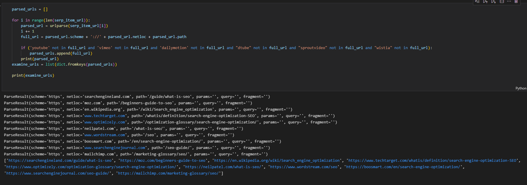
- Print the URLs to be examined.
You can see the result below.
 Screenshot from author, August 2022
4. Crawl The Cleaned Examine URLs For Retrieving Their Content
Crawl the cleaned examine URLs for retrieving their content with advertools.
You can also use requests with a for loop and list append methodology, but advertools is faster for crawling and creating the data frame with the resulting output.
With requests, you manually retrieve and unite all the “p” and “heading” elements.
adv.crawl(examine_urls, output_file="examine_urls.jl",

          follow_links=False,

          custom_settings={"USER_AGENT": UserAgent().random,

                           "LOG_FILE": "examine_urls.log",

                           "CRAWL_DELAY": 2})

crawled_df = pd.read_json("examine_urls.jl", lines=True)

crawled_df
Explanation of code block above:
- Use “adv.crawl” for crawling the “examine_urls” object.
- Create a path for output files with “jl” extension, which is smaller than others.
- Use “follow_links=false” to stop crawling only for listed URLs.
- Use custom settings to state a “random user agent” and a crawl log file if some URLs do not answer the crawl requests. Use a crawl delay configuration to prevent 429 status code possibility.
- Use pandas “read_json” with the “lines=True” parameter to read the results.
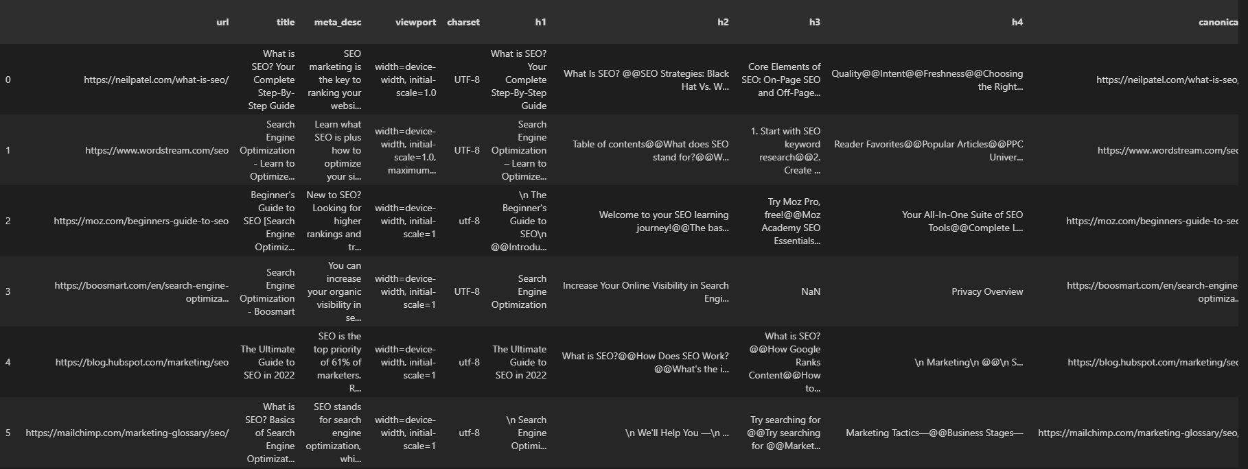
- Call the “crawled_df” as below.
You can see the result below.
 Screenshot from author, August 2022
You can see our result URLs and all their on-page SEO elements, including response headers, response sizes, and structured data information.
5. Tokenize The Content Of The Web Pages For Text Processing In NLP Methodologies
Tokenization of the content of the web pages requires choosing the “body_text” column of advertools crawl output and using the “word_tokenize” from NLTK.
crawled_df["body_text"][0]The code line above calls the entire content of one of the result pages as below.
 Screenshot from author, August 2022
To tokenize these sentences, use the code block below.
tokenized_words = word_tokenize(crawled_df["body_text"][0])

len(tokenized_words)
We tokenized the content of the first document and checked how many words it had.
 Screenshot from author, August 2022
The first document we tokenized for the query “search engine optimization” has 11211 words. And boilerplate content is included in this number.
6. Remove The Punctuations And Stop Words From Corpus
Remove the punctuations, and the stop words, as below.
stop_words = set(stopwords.words("english"))
tokenized_words = [word for word in tokenized_words if not word.lower() in stop_words and word.lower() not in string.punctuation]

len(tokenized_words)
Explanation of code block above:
- Create a set with the “stopwords.words(“english”)” to include all the stop words in the English language. Python sets do not include duplicate values; thus, we used a set rather than a list to prevent any conflict.
- Use list comprehension with “if” and “else” statements.
- Use the “lower” method to compare the “And” or “To” types of words properly to their lowercase versions in the stop words list.
- Use the “string” module and include “punctuations.” A note here is that the string module might not include all the punctuations that you might need. For these situations, create your own punctuation list and replace these characters with space using the regex, and “regex.sub.”
- Optionally, to remove the punctuations or some other non-alphabetic and numeric values, you can use the “isalnum” method of Python strings. But, based on the phrases, it might give different results. For example, “isalnum” would remove a word such as “keyword-related” since the “-” at the middle of the word is not alphanumeric. But, string.punctuation wouldn’t remove it since “keyword-related” is not punctuation, even if the “-” is.
- Measure the length of the new list.
The new length of our tokenized word list is “5319”. It shows that nearly half of the vocabulary of the document consists of stop words or punctuations.
It might mean that only 54% of the words are contextual, and the rest is functional.
7. Count The Number Of Occurrences Of The Words In The Content Of The Web Pages
To count the occurrences of the words from the corpus, the “Counter” object from the “Collections” module is used as below.
counted_tokenized_words = Counter(tokenized_words)

counts_of_words_df = pd.DataFrame.from_dict(

    counted_tokenized_words, orient="index").reset_index()

counts_of_words_df.sort_values(by=0, ascending=False, inplace=True)

counts_of_words_df.head(50)
An explanation of the code block is below.
- Create a variable such as “counted_tokenized_words” to involve the Counter method results.
- Use the “DataFrame” constructor from the Pandas to construct a new data frame from Counter method results for the tokenized and cleaned text.
- Use the “from_dict” method because “Counter” gives a dictionary object.
- Use “sort_values” with “by=0” which means sort based on the rows, and “ascending=False” means to put the highest value to the top. “Inpace=True” is for making the new sorted version permanent.
- Call the first 50 rows with the “head()” method of pandas to check the first look of the data frame.
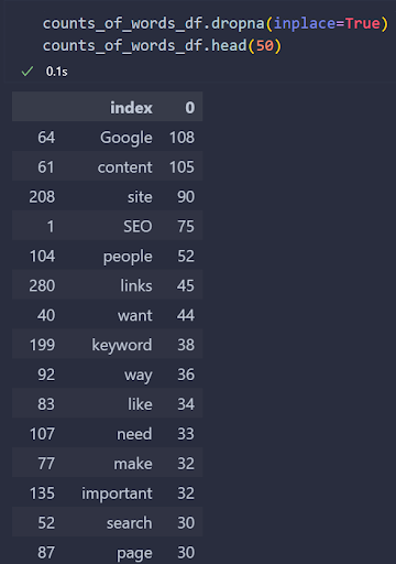
You can see the result below.
 Screenshot from author, August 2022
We do not see a stop word on the results, but some interesting punctuation marks remain.
That happens because some websites use different characters for the same purposes, such as curly quotes (smart quotes), straight single quotes, and double straight quotes.
And string module’s “functions” module doesn’t involve those.
Thus, to clean our data frame, we will use a custom lambda function as below.
removed_curly_quotes = "’“”"

counts_of_words_df["index"] = counts_of_words_df["index"].apply(lambda x: float("NaN") if x in removed_curly_quotes else x)

counts_of_words_df.dropna(inplace=True)

counts_of_words_df.head(50)
Explanation of code block:
- Created a variable named “removed_curly_quotes” to involve a curly single, double quotes, and straight double quotes.
- Used the “apply” function in pandas to check all columns with those possible values.
- Used the lambda function with “float(“NaN”) so that we can use “dropna” method of Pandas.
- Use “dropna” to drop any NaN value that replaces the specific curly quote versions. Add “inplace=True” to drop NaN values permanently.
- Call the dataframe’s new version and check it.
You can see the result below.
 Screenshot from author, August 2022
We see the most used words in the “Search Engine Optimization” related ranking web document.
With Panda’s “plot” methodology, we can visualize it easily as below.
counts_of_words_df.head(20).plot(kind="bar",x="index", orientation="vertical", figsize=(15,10), xlabel="Tokens", ylabel="Count", colormap="viridis", table=False, grid=True, fontsize=15, rot=35, position=1, title="Token Counts from a Website Content with Punctiation", legend=True).legend(["Tokens"], loc="lower left", prop={"size":15})Explanation of code block above:
- Use the head method to see the first meaningful values to have a clean visualization.
- Use “plot” with the “kind” attribute to have a “bar plot.”
- Put the “x” axis with the columns that involve the words.
- Use the orientation attribute to specify the direction of the plot.
- Determine figsize with a tuple that specifies height and width.
- Put x and y labels for x and y axis names.
- Determine a colormap that has a construct such as “viridis.”
- Determine font size, label rotation, label position, the title of plot, legend existence, legend title, location of legend, and size of the legend.
The Pandas DataFrame Plotting is an extensive topic. If you want to use the “Plotly” as Pandas visualization back-end, check the Visualization of Hot Topics for News SEO.
You can see the result below.
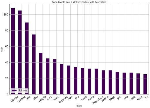 Image from author, August 2022
Now, we can choose our second URL to start our comparison of vocabulary size and occurrence of words.
8. Choose The Second URL For Comparison Of The Vocabulary Size And Occurrences Of Words
To compare the previous SEO content to a competing web document, we will use SEJ’s SEO guide. You can see a compressed version of the steps followed until now for the second article.
def tokenize_visualize(article:int):

    stop_words = set(stopwords.words("english"))

    removed_curly_quotes = "’“”"

    tokenized_words = word_tokenize(crawled_df["body_text"][article])

    print("Count of tokenized words:", len(tokenized_words))

    tokenized_words = [word for word in tokenized_words if not word.lower() in stop_words and word.lower() not in string.punctuation and word.lower() not in removed_curly_quotes]

    print("Count of tokenized words after removal punctations, and stop words:", len(tokenized_words))

    counted_tokenized_words = Counter(tokenized_words)

    counts_of_words_df = pd.DataFrame.from_dict(

    counted_tokenized_words, orient="index").reset_index()

    counts_of_words_df.sort_values(by=0, ascending=False, inplace=True)

    #counts_of_words_df["index"] = counts_of_words_df["index"].apply(lambda x: float("NaN") if x in removed_curly_quotes else x)

    counts_of_words_df.dropna(inplace=True)

    counts_of_words_df.head(20).plot(kind="bar",

    x="index",

    orientation="vertical",

    figsize=(15,10),

    xlabel="Tokens",

    ylabel="Count",

    colormap="viridis",

    table=False,

    grid=True,

    fontsize=15,

    rot=35,

    position=1,

    title="Token Counts from a Website Content with Punctiation",

    legend=True).legend(["Tokens"],

    loc="lower left",

    prop={"size":15})
We collected everything for tokenization, removal of stop words, punctations, replacing curly quotations, counting words, data frame construction, data frame sorting, and visualization.
Below, you can see the result.
 Screenshot by author, August 2022
The SEJ article is in the eighth ranking.
tokenize_visualize(8)The number eight means it ranks eighth on the crawl output data frame, equal to the SEJ article for SEO. You can see the result below.
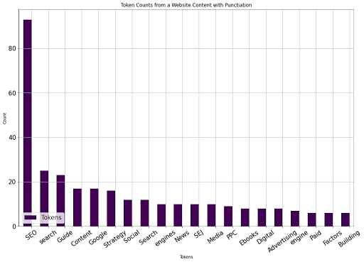 Image from author, August 2022
We see that the 20 most used words between the SEJ SEO article and other competing SEO articles differ.
9. Create A Custom Function To Automate Word Occurrence Counts And Vocabulary Difference Visualization
The fundamental step to automating any SEO task with Python is wrapping all the steps and necessities under a certain Python function with different possibilities.
The function that you will see below has a conditional statement. If you pass a single article, it uses a single visualization call; for multiple ones, it creates sub-plots according to the sub-plot count.
def tokenize_visualize(articles:list, article:int=None):

     if article:

          stop_words = set(stopwords.words("english"))

          removed_curly_quotes = "’“”"

          tokenized_words = word_tokenize(crawled_df["body_text"][article])

          print("Count of tokenized words:", len(tokenized_words))

          tokenized_words = [word for word in tokenized_words if not word.lower() in stop_words and word.lower() not in string.punctuation and word.lower() not in removed_curly_quotes]

          print("Count of tokenized words after removal punctations, and stop words:", len(tokenized_words))

          counted_tokenized_words = Counter(tokenized_words)

          counts_of_words_df = pd.DataFrame.from_dict(

          counted_tokenized_words, orient="index").reset_index()

          counts_of_words_df.sort_values(by=0, ascending=False, inplace=True)

          #counts_of_words_df["index"] = counts_of_words_df["index"].apply(lambda x: float("NaN") if x in removed_curly_quotes else x)

          counts_of_words_df.dropna(inplace=True)

          counts_of_words_df.head(20).plot(kind="bar",

          x="index",

          orientation="vertical",

          figsize=(15,10),

          xlabel="Tokens",

          ylabel="Count",

          colormap="viridis",

          table=False,

          grid=True,

          fontsize=15,

          rot=35,

          position=1,

          title="Token Counts from a Website Content with Punctiation",

          legend=True).legend(["Tokens"],

          loc="lower left",

          prop={"size":15})


     if articles:

          source_names = []

          for i in range(len(articles)):

               source_name = crawled_df["url"][articles[i]]

               print(source_name)

               source_name = urlparse(source_name)

               print(source_name)

               source_name = source_name.netloc

               print(source_name)

               source_names.append(source_name)

          global dfs

          dfs = []

          for i in articles:

               stop_words = set(stopwords.words("english"))

               removed_curly_quotes = "’“”"

               tokenized_words = word_tokenize(crawled_df["body_text"][i])

               print("Count of tokenized words:", len(tokenized_words))

               tokenized_words = [word for word in tokenized_words if not word.lower() in stop_words and word.lower() not in string.punctuation and word.lower() not in removed_curly_quotes]

               print("Count of tokenized words after removal punctations, and stop words:", len(tokenized_words))

               counted_tokenized_words = Counter(tokenized_words)

               counts_of_words_df = pd.DataFrame.from_dict(

               counted_tokenized_words, orient="index").reset_index()

               counts_of_words_df.sort_values(by=0, ascending=False, inplace=True)

               #counts_of_words_df["index"] = counts_of_words_df["index"].apply(lambda x: float("NaN") if x in removed_curly_quotes else x)

               counts_of_words_df.dropna(inplace=True)

               df_individual = counts_of_words_df

               dfs.append(df_individual)


          import matplotlib.pyplot as plt

          figure, axes = plt.subplots(len(articles), 1)

          for i in range(len(dfs) + 0):

               dfs[i].head(20).plot(ax = axes[i], kind="bar",

                    x="index",

                    orientation="vertical",

                    figsize=(len(articles) * 10, len(articles) * 10),

                    xlabel="Tokens",

                    ylabel="Count",

                    colormap="viridis",

                    table=False,

                    grid=True,

                    fontsize=15,

                    rot=35,

                    position=1,

                    title= f"{source_names[i]} Token Counts",

                    legend=True).legend(["Tokens"],

                    loc="lower left",

                    prop={"size":15})
To keep the article concise, I won’t add an explanation for those. Still, if you check previous SEJ Python SEO tutorials I have written, you will realize similar wrapper functions.
Let’s use it.
tokenize_visualize(articles=[1, 8, 4])
We wanted to take the first, eighth, and fourth articles and visualize their top 20 words and their occurrences; you can see the result below.
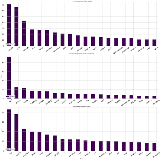 Image from author, August 2022
10. Compare The Unique Word Count Between The Documents
Comparing the unique word count between the documents is quite easy, thanks to pandas. You can check the custom function below.
def compare_unique_word_count(articles:list):

     source_names = []

     for i in range(len(articles)):

          source_name = crawled_df["url"][articles[i]]

          source_name = urlparse(source_name)

          source_name = source_name.netloc

          source_names.append(source_name)


     stop_words = set(stopwords.words("english"))

     removed_curly_quotes = "’“”"

     i = 0

     for article in articles:

          text = crawled_df["body_text"][article]

          tokenized_text = word_tokenize(text)

          tokenized_cleaned_text = [word for word in tokenized_text if not word.lower() in stop_words if not word.lower() in string.punctuation if not word.lower() in removed_curly_quotes]

          tokenized_cleanet_text_counts = Counter(tokenized_cleaned_text)

          tokenized_cleanet_text_counts_df = pd.DataFrame.from_dict(tokenized_cleanet_text_counts, orient="index").reset_index().rename(columns={"index": source_names[i], 0: "Counts"}).sort_values(by="Counts", ascending=False)

          i += 1

          print(tokenized_cleanet_text_counts_df, "Number of unique words: ",  tokenized_cleanet_text_counts_df.nunique(), "Total contextual word count: ", tokenized_cleanet_text_counts_df["Counts"].sum(), "Total word count: ", len(tokenized_text))

compare_unique_word_count(articles=[1, 8, 4])
The result is below.
The bottom of the result shows the number of unique values, which shows the number of unique words in the document.
www.wordstream.com Counts
16 Google 71
82 SEO 66
186 search 43
228 site 28
274 page 27
… … …
510 markup/structured 1
1 Recent 1
514 mistake 1
515 bottom 1
1024 LinkedIn 1
[1025 rows x 2 columns] Number of unique words:
www.wordstream.com 1025
Counts 24
dtype: int64 Total contextual word count: 2399 Total word count: 4918
www.searchenginejournal.com Counts
9 SEO 93
242 search 25
64 Guide 23
40 Content 17
13 Google 17
.. … …
229 Action 1
228 Moving 1
227 Agile 1
226 32 1
465 news 1
[466 rows x 2 columns] Number of unique words:
www.searchenginejournal.com 466
Counts 16
dtype: int64 Total contextual word count: 1019 Total word count: 1601
blog.hubspot.com Counts
166 SEO 86
160 search 76
32 content 46
368 page 40
327 links 39
… … …
695 idea 1
697 talked 1
698 earlier 1
699 Analyzing 1
1326 Security 1
[1327 rows x 2 columns] Number of unique words:
blog.hubspot.com 1327
Counts 31
dtype: int64 Total contextual word count: 3418 Total word count: 6728
There are 1025 unique words out of 2399 non-stopword and non-punctuation contextual words. The total word count is 4918.
The most used five words are “Google,” “SEO,” “search,” “site,” and “page” for “Wordstream.” You can see the others with the same numbers.
11. Compare The Vocabulary Differences Between The Documents On The SERP
Auditing what distinctive words appear in competing documents helps you see where the document weighs more and how it creates a difference.
The methodology is simple: “set” object type has a “difference” method to show the different values between two sets.
def audit_vocabulary_difference(articles:list):

     stop_words = set(stopwords.words("english"))

     removed_curly_quotes = "’“”"

     global dfs

     global source_names

     source_names = []

     for i in range(len(articles)):

          source_name = crawled_df["url"][articles[i]]

          source_name = urlparse(source_name)

          source_name = source_name.netloc

          source_names.append(source_name)

     i = 0

     dfs = []

     for article in articles:

               text = crawled_df["body_text"][article]

               tokenized_text = word_tokenize(text)

               tokenized_cleaned_text = [word for word in tokenized_text if not word.lower() in stop_words if not word.lower() in string.punctuation if not word.lower() in removed_curly_quotes]

               tokenized_cleanet_text_counts = Counter(tokenized_cleaned_text)

               tokenized_cleanet_text_counts_df = pd.DataFrame.from_dict(tokenized_cleanet_text_counts, orient="index").reset_index().rename(columns={"index": source_names[i], 0: "Counts"}).sort_values(by="Counts", ascending=False)

               tokenized_cleanet_text_counts_df.dropna(inplace=True)

               i += 1

               df_individual = tokenized_cleanet_text_counts_df

               dfs.append(df_individual)

     global vocabulary_difference

     vocabulary_difference = []

     for i in dfs:

          vocabulary = set(i.iloc[:, 0].to_list())

          vocabulary_difference.append(vocabulary)

     print( "Words that appear on :", source_names[0], "but not on: ", source_names[1], "are below: \n", vocabulary_difference[0].difference(vocabulary_difference[1]))
To keep things concise, I won’t explain the function lines one by one, but basically, we take the unique words in multiple articles and compare them to each other.
You can see the result below.
Words that appear on: www.techtarget.com but not on: moz.com are below:
 Screenshot by author, August 2022
Use the custom function below to see how often these words are used in the specific document.
def unique_vocabulry_weight():

     audit_vocabulary_difference(articles=[3, 1])

vocabulary_difference_list = vocabulary_difference_df[0].to_list()

     return dfs[0][dfs[0].iloc[:, 0].isin(vocabulary_difference_list)]

unique_vocabulry_weight()
The results are below.
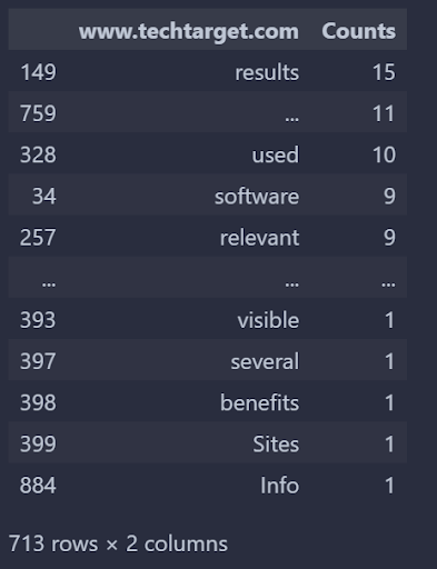 Screenshot by author, August 2022
The vocabulary difference between TechTarget and Moz for the “search engine optimization” query from TechTarget’s perspective is above. We can reverse it.
def unique_vocabulry_weight():

audit_vocabulary_difference(articles=[1, 3])

vocabulary_difference_list = vocabulary_difference_df[0].to_list()

return dfs[0][dfs[0].iloc[:, 0].isin(vocabulary_difference_list)]

unique_vocabulry_weight()
Change the order of numbers. Check from another perspective.
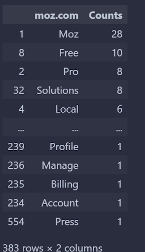 Screenshot by author, August 2022
You can see that Wordstream has 868 unique words that do not appear on Boosmart, and the top five and tail five are given above with their occurrences.
The vocabulary difference audit can be improved with “weighted frequency” by checking the query information and network.
But, for teaching purposes, this is already a heavy, detailed, and advanced Python, Data Science, and SEO intensive course.
See you in the next guides and tutorials.
More resources:
Featured Image: VectorMine/Shutterstock
 seolounge